Picking a TTL under Exponential Changes

March 28, 2026

This post derives a closed-form way to choose a cache TTL from a target staleness budget when underlying data changes follow an exponential model.

Introduction

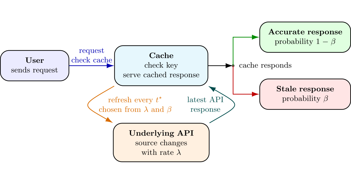
Suppose we’re maintaining a cache in front of an API endpoint whose responses can change over time. In this post, we assume a fixed refresh policy: once an entry is written or refreshed, we revalidate it exactly \(t\) time units later. A longer TTL means fewer refreshes, but it also increases the chance of serving stale data. A shorter TTL improves freshness, but forces more frequent refreshes.

For each cache entry, we want to choose the largest TTL that still keeps expected staleness below an acceptable threshold. If one refresh costs one unit, then a fixed TTL of length \(t\) induces a refresh cost rate of \(1/t\), so the largest admissible TTL is also the cheapest one. Here’s the trade-off:

• If the TTL is too low, entries are refreshed more often than necessary.
• If the TTL is too high, entries remain cached after the underlying data has changed.

We’ll derive the formula for a single cache entry and then apply it entry-by-entry. One entry might deserve TTL = 1h while another can safely use TTL = 2h, depending on how often its source data changes. Under an exponential change model, this TTL can be computed in closed form.

Problem Statement

Fix a single cache entry. Let \(t>0\) be its TTL, let \(\lambda>0\) be the rate at which the underlying value changes, and let \(T\) denote the time from a refresh until the next underlying change. We first derive the stale fraction for this one entry, then reuse the same formula for every other entry with its own \(\lambda\).

Let’s assume the underlying API endpoint updates its results every once in a while, based on a Poisson process. As the Poisson process is memoryless, the time \(T\) until the next change is an exponential variable:

The exact moment of change is stochastic, so freshness is never certain. The goal is to choose a deterministic TTL \(t\) that controls the expected stale fraction under this model.

Even though we’ll never know for sure whether the entry is stale at a given moment, we can quantify its expected stale fraction over a TTL cycle.

How To Measure Staleness

Fix a single cache cycle of length \(t>0\), starting when the entry is written or refreshed. Let \(T\) be the time until the underlying data changes next. Two cases can happen during that cycle:

• If \(T \ge t\), the data does not change before the cache is refreshed, so the entry stays fresh for the entire cycle and contributes zero staleness.
• If \(T < t\), the data changes before refresh, so the entry is fresh on \([0,T]\) and stale on \([T,t]\), contributing stale duration \(t - T\).

Both cases are captured compactly by saying the stale duration in one cycle is \((t-T)^+\), where the positive-part operator clips negative values to zero. Dividing by the cycle length \(t\) gives the stale fraction of that cycle:

First let’s simplify \(\mathbb{E}\!\left[(t-T)^+\right]\):

The \( \mathbb{E}\!\left[ T \mid T\le t \right] \) is the expectation of a truncated exponential distribution. Therefore:

Now that \(\mathbb{E}\!\left[(t-T)^+\right]\) is simplified, \(S(t)\) can be derived:

Pick the TTL from a Staleness Budget

Suppose you choose a per-entry staleness budget \(\beta\in[0,1)\), meaning you require

Assume each refresh costs one unit. Under a fixed TTL \(t\), one refresh happens every \(t\) time units, so the long-run refresh cost rate is \(1/t\). Therefore, among all TTLs satisfying the staleness budget, the cheapest choice is the largest feasible one.

Since \(S(t)\) increases with \(t\), the largest admissible TTL is the unique solution of

Set \(S(t)=\beta\) and solve for \(t\). Let \(y\coloneqq \lambda t^\star\):

The function \(\frac{1 - e^{-y}}{y}\) can be inverted using the Lambert \(W\) function:

This gives the largest TTL whose expected stale fraction is at most \(\beta\).

Worked Example

Suppose an entry changes on average once every 5 days, so \(\lambda = 0.2\) per day, and you want expected staleness no higher than 10%, so \(\beta = 0.1\). Plugging those into the formula gives

So in this case, a TTL of about 26 hours is the largest fixed refresh interval that keeps expected stale time within the 10% budget under the model.

Python Implementation

Here’s a simple Python implementation using scipy for the Lambert-\(W\) function:

import numpy as np
from scipy.special import lambertw

def compute_ttl(lambda_rate, staleness_budget):
    """Return the largest TTL whose expected stale fraction stays within budget.

    Assumes the underlying data changes according to an exponential waiting-time
    model with rate ``lambda_rate`` and that ``staleness_budget`` is in ``[0, 1)``.
    """
    if lambda_rate <= 0:
        raise ValueError("lambda_rate must be positive")
    if not 0 <= staleness_budget < 1:
        raise ValueError("staleness_budget must be in [0, 1)")

    freshness_target = 1 - staleness_budget
    lambert_w_input = -1 / freshness_target * np.exp(-1 / freshness_target)
    return (1 / lambda_rate) * (
        lambertw(lambert_w_input).real + 1 / freshness_target
    )

Quick Reference

The Model

• Change process: \(T\sim\mathrm{Exp}(\lambda)\) where \(\lambda > 0\) is the change rate
• Refresh policy: refresh exactly every \(t\) time units
• Refresh cost rate: \(1/t\) if each refresh costs one unit

Key Formulas

• Staleness function: \(S(t)=1-\dfrac{1-e^{-\lambda t}}{\lambda t}\)
• Optimal TTL: Given staleness budget \(\beta\in[0,1)\), choose

Decision Process

1. Estimate change rates from historical data. Different entities might have different \(\lambda\) values, but a single global \(\lambda\) can also work if their behavior is similar.
2. Determine an acceptable stale fraction \(\beta\) based on business requirements
3. Compute optimal TTLs using the Lambert \(W\) formula
4. Monitor actual staleness and adjust the \(\lambda\) estimates if needed